Abstract
A machine learning approach using image features can accurately classify monkeypox skin lesions with high accuracy.
Researchers developed a machine learning system that uses image features to classify monkeypox skin lesions. They extracted texture features from images using various techniques and applied a data balancing method to improve accuracy. The system achieved high accuracy, with the Random Forest classifier performing best, and highlighted the potential of image-based classification for detecting monkeypox.
Full TextOpen Access
The poxviridae family consists of complex, double-stranded, DNA-containing viruses that are divided into two subfamilies: Chondropoxvirinae (those infecting vertebrates), and Entomopoxvirinae (those infecting insects) [1], [2]. One of the genera in the Chondropoxvirinae subfamily is Orthopoxvirus, which causes several human diseases [3], [4]. Examples of these human illnesses are variola (smallpox) [5], monkeypox, and cowpox [3].
Unlike smallpox, which was eradicated in 1980, monkeypox continues to cause serious global health concerns as it continues to occur in several parts of the world [6]. It was first discovered in monkeys in 1959 at a Danish research facility [7], [8]. It was later found to have infected humans in the Democratic Republic of Congo (DRC) in 1970 [9]. Monkeypox has mostly been confined to West and Central African countries such as Nigeria, the Central African Republic, Liberia, Sierra Leone, and Cameroon, while the first outbreak outside Africa occurred in the United States in 2003. The increasing number of monkeypox cases in various regions of the world, including nonendemic countries was reported by the World Health Organization (WHO), which confirmed 82,809 cases in 110 countries by the end of 2022 [9], [10]. The monkeypox virus can spread rapidly from human to human through contact with the blood, body fluids, contaminated materials or physical contact with an infected person. It can also be transmitted through contact with an infected animal, its bite, or scratch [11], [12], [13]. Symptoms include fever, chills, headache, body aches, muscle pain, fatigue, and swollen lymph nodes, which are similar to those of flu and smallpox [14]. As the disease progresses, it develops rashes red, painful papules which gradually turn into pus-filled blisters. Monkeypox is difficult to diagnose early because of its similar symptoms with other diseases (such as; scarlet fever, roseola and smallpox) [15]. Although diagnosis through PCR testing and treatment with the chickenpox vaccine have been attempted, the rapid identification and differentiation of the disease are crucial for its treatment and containment.
For these reasons, the goal is to automatically diagnose the illness using machine learning (ML) and deep learning (DL) techniques along with other artificial intelligence techniques, like image analysis, which are known to be effective in differentiating between various diseases.
In the literature, there are many studies focused on diagnosing and classifying monkeypox virus from images. For instance, Ahsan et al. [16], conducted their research using the publicly available “Monkeypox2022” dataset [17]. Their study was carried out in two phases: the first phase focused on classifying monkeypox and chickenpox while the second phase involved classifying augmented monkeypox and other diseases. A modified VGG-16 model was proposed for classification. With this model, they achieved an AUC of 97.2% in the first phase and 74.8% in the second phase. Sitaula ve Shahi [18], used the same dataset collected by Ahsan et al. [17] and applied Xception transfer learning with Grad-Cam and LIME techniques. A combined ensemble approach using Xception and DenseNet models was designed. This approach achieved an average precision of 85.44%, recall of 85.47%, F1 score of 85.40% and an accuracy of 87.13%. Ali et al. [19], using the same dataset, applied data augmentation techniques with three-fold cross-validation. The study evaluated the performance of pre-trained VGG-16, ResNet50, and InceptionV3 models for classifying monkeypox and other diseases. Among these models, ResNet50 achieved the highest accuracy of 82.96% (±4.57).
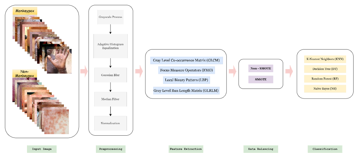
In another study by Islam et al. [20], the detectability of monkeypox from digital skin images using artificial intelligence was investigated. The dataset consisted of six groups (Monkeypox, Chickenpox, Smallpox, Cowpox, Measles, and healthy skin). Seven different models were applied, including ResNet50, DenseNet21, Inception-V3, Squeeze Net, MnasNet-AI, MobileNet-V2 and ShuffleNet-V2-1X achieving an average accuracy of 83%. Another paper [21] presented a study on "Human Monkeypox Classification from Skin Lesions Using Pre-trained Deep Network Models via a Mobile Application." In this study, image data were processed on an Android-based mobile application using transfer learning techniques. The researchers performed classification using NasNetMobile, ResNet18, GoogleNet, ShuffleNet, EfficientNetb0 and MobileNetv2 models on the dataset from Ali et al. [19]. The best result was obtained with the MobileNetv2 model achieving 91% accuracy and 90% F1 score. In the current study, we aimed to develop a high-performance classification model using the publicly available Monkeypox Skin Lesion Dataset (MSLD) [19] from Kaggle. The MSLD dataset consists of two classes: Monkeypox and Non-Monkeypox. Images were analyzed in both their raw form and after preprocessing steps. The preprocessing phase made the data suitable for feature extraction and various features were calculated to enhance classification performance. The preprocessed images were used to extract features such as Gray Level Co-Occurrence Matrix (GLCM), Gray Level Run Length Matrix (GLRLM), Focus Measure Operators (FMOs), and Local Binary Pattern (LBP). To guarantee data balance between the Monkeypox and non-Monkeypox classes, the Synthetic Minority Oversampling Technique (SMOTE) algorithm was employed. The computed features' classification performance for differentiating
K-Nearest Neighbors (KNN), Decision Trees (DT), Random Forest (RF), and Naive Bayes (NB) machine learning techniques were used to assess the differences between Monkeypox and non-Monkeypox groups.
Other studies related to the monkeypox virus are shown in Table 1. In the study, a high-performance classification model was developed by primarily implementing the following key steps listed below.
· Comprehensive Feature Analysis: As a result of comprehensive analyses conducted on Monkeypox and non-Monkeypox datasets, distinguishable new information was obtained using texture-based feature extraction methods such as GLCM, GLRLM, FMOs and LBP. Thus, distinctive features related to monkeypox disease were analyzed.
· Data Balancing with the SMOTE Algorithm: To effectively address data imbalance, a detailed analysis was conducted on the existing dataset using the SMOTE.
· Feature Selection with LASSO (Least Absolute Shrinkage and Selection Operator) Regression: Using the LASSO method, optimal features were determined by testing different parameter values and selecting those that yielded the lowest Mean Squared Error (MSE) result.
· Efficient Classification with Machine Learning: The chosen features were then classified using advanced machine learning algorithms that would make the difference between data groups robust as well as accurate.
This research involved analyzing Monkeypox and Non-Monkeypox images that are available on the publicly accessible Kaggle site. After preprocessing, we extracted features using texture-based approaches such as GLCM, GLRLM, FMOs, and LBP. Then we employed the SMOTE algorithm to adjust the number of samples in the Monkeypox and Non-Monkeypox groups. Each of these steps were carried out separately on both non-augmented and augmented datasets. Finally, we trialed various machine learning techniques, to evaluate the outputs of our selected features and classify monkeypox vs. non-monkeypox. The classification process was achieved over three phases: classification of each feature individually, classification of all features cumulatively, and selecting the most optimal features using the LASSO method. The flow chart of the proposed study is shown in Figure 1.
Author(s), Year | Database and classes | Classification Method | Result |
Matuszewski et al. [22], 2021 | 1245 images of 22 diferent virus classes | DenseNet201 | 93.1% Accuracy |
Ahsan et al.[16], 2022 | Normal, Chickenpox, Monkeypox, Measles Monkeypox-dataset-2022 [17] | VGG16-based transfer learning | Study One: 97% ± 1.8 Accuracy (AUC = 97.2) Study Two: 88% ± 0.8 Accuracy (AUC = 0.867) |
Abdelhamid et al.[23], 2022 | Normal, Monkeypox from Kaggle | Neural network | 98.8 % Accuracy |
Singh et al.[24], 2022 | Kaggle dataset | GoogLeNet model | 88.27% Accuracy |
Ali et al.[19], 2022 | MSLD database [19] | ResNet50, VGG-16, and InceptionV3 | ResNet50- 82.96% (±4.57), VGG16 - 81.48% (±6.87), Inception V3 - 74.07% (±3.78) Accuracy |
Sahin et al.[21], 2022 | MSLD database [19] | MobileNetv2 model | 91.11% Accuracy |
Sitaula and Shahi [18], 2022 | Normal, Chickenpox, Monkeypox, Measles Monkeypox-dataset-2022 [17] | Ensemble pretrained deep learning | 87.13 % Accuracy |
Islam et al.[20], 2022 | Normal, Monkeypox, Smallpox, Chickenpox, Cowpox, Measles | ShuffleNet-V2 and Ensemble CNN | 83.0 % Accuracy |
Dwivedi et al.[25], 2023 | Kaggle Monkeypox dataset | ResNet5 model | 87% Accuracy |
Kumar [26], 2022 | MSLD database [19] | AlexNet, GoogleNet and VGG16Net (CNN models), SVM, NB, KNN, RF, and DT (machine learning models) | 91.11% Accuracy |
Saleh et al.[27],2023 | Monkeypox dataset | Weighted Naïve Bayes (WNB) | 92.56% Accuracy |
Benges et al.[28], 2023 | 500,000 Monkeypox Twitters | SVM model | 93.48% Accuracy |
Bala et al.[29], 2023 | Normal, Chickenpox, Monkeypox, Measles from Kaggle | Classical machine learning classifiers and CNN | Test-1: 93.19 % Accuracy Test-2: 98.91% Accuracy |
Ozsahin et al.[12], 2023 | Monkeypox/Chickenpox from Kaggle [19] | CNN | 99.60 % Accuracy |
Yasmin et al.[30], 2023 | Monkeypox/Non-monkeypox from Kaggle [19] | PoxNet22 (custom designed CNN) | 100 % Accuracy |
Dataset
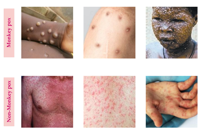
The data used in this study were obtained from the Monkeypox Skin Lesion Dataset (MSLD) [19], which is publicly available on the Kaggle platform. All data used in this study were obtained from publicly available and anonymized datasets. As no human participants were directly involved and no identifiable personal data were used, ethical approval was not required in accordance with institutional and national guidelines. The dataset contains a total of 228 images, of which 102 are classified as Monkeypox and 126 as non-Monkeypox (Others). Each image has a resolution of 224 × 224 pixels. The ‘Monkeypox’ group consists of skin lesion images of individuals with monkeypox, while the non-Monkeypox group contains skin lesion images from diseases such as chickenpox or measles, which share similar features with monkeypox. Some sample images from the dataset are shown in Figure 2.
Preprocessing
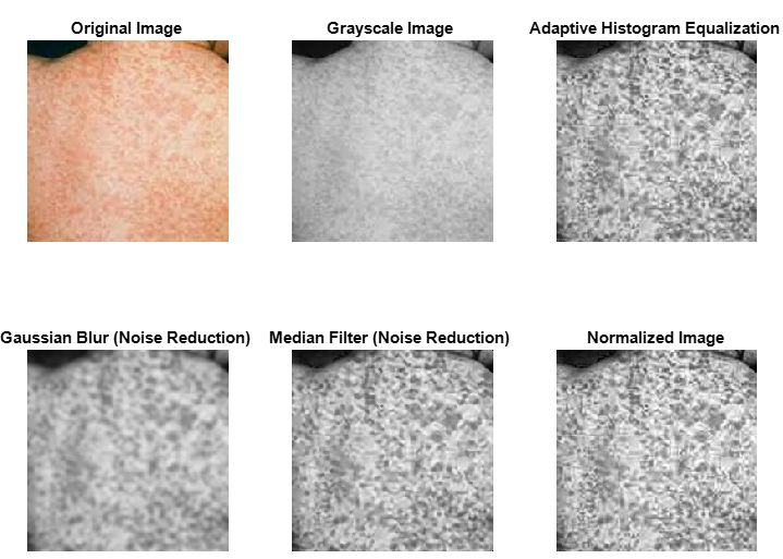
In this study, several image preprocessing methods were used to enhance image analysis and classification. These included Gaussian blur to smooth the image and reduce noise, median filtering to get rid of salt-and-pepper noise, and adaptive histogram equalization to improve contrast and highlight details in low light. Additionally, normalization was used to ensure consistency between images by standardizing pixel values within the 0–255 range. The goal of these preprocessing procedures was to improve model performance for tasks like feature extraction and classification. Figure 3 shows the preprocessing steps performed on a sample image. Notably, no segmentation process was performed, as the goal was to develop a system capable of analyzing user-uploaded images and determining whether they were monkeypox virus cases using machine-learning algorithms without requiring segmentation through expert knowledge.
Synthetic Minority Oversampling Technique (SMOTE)
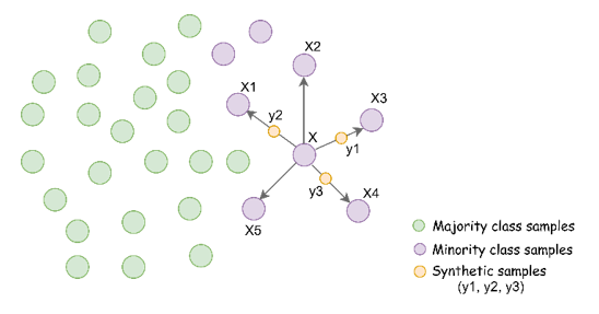
The SMOTE is one of the most widely used sampling methods. Developed in 2002, this algorithm has been presented as a solution for many imbalanced dataset problems [31], [32], [33]. The SMOTE algorithm generates synthetic samples by using the neighborhood relationships among samples in the minority class rather than simply replicating them. This method reduces learning problems caused by class imbalance and enables classification models to make more balanced and reliable predictions. The working mechanism of the algorithm is shown in Figure 4.
Steps of the algorithm:
1. The k-nearest neighbors are searching for each sample in the minority class.
2. The difference between the minority class sample and its k-nearest neighbor is calculated,
3. (A random number (α) between 0 and 1 is selected and multiplied by the difference found in Step b,
4. A new synthetic sample is generated using Equation (1).
5. The steps are repeated until the desired number of synthetic samples is created.
(1)
In this study, the SMOTE algorithm was applied as a preprocessing step to eliminate data imbalance and improve the performance of classification algorithms. The balanced data groups, after the application of the SMOTE algorithm on the dataset, were used in the analysis and modeling. This was one of the ways through which the low sensitivity issues in imbalanced data datasets could be reduced, especially for the minority class, and performance improved. The comparison of model performance before and after balancing was made. Table 2 gives the number of images in the dataset.
Unbalanced | Balanced | |||
|---|---|---|---|---|
Data | Monkey pox | Non-Monkey pox | Monkey pox | Non-Monkey pox |
Non-augmented | 102 | 126 | 126 | 126 |
Augmented | 1428 | 1764 | 1764 | 1764 |
Feature Extraction
Different features extraction approaches were used to give a more detailed analysis of the textural and structural properties of the lesions in the image data and to enhance classification performance. Ensemble methods included GLCM, GLRLM, FMO, and LBP types. The GLCM extracts the texture-specific parameters based on the spatial relationship of pixels in an image. It measures texture properties, including contrast, energy, and homogeneity. It is the Gray Level Run Length Matrix that computes the run length between pixel groups concerning the same gray level to extract texture regularity and repetitiveness. FMOs calculate the focus measures in an image refocusing and clarify lesions. These methods allow for extracting useful and discriminative features from given raw image data. Besides reducing the data size, it is aimed at enhancing the accuracy and efficiency of classification algorithms, hence facilitating better analysis of lesions for a classification task.
Focus Measure Operators (FMOs)
FMOs are one of the major features of extraction methods in image processing and analysis. FMOs are developed for quantitatively measuring the level of focus or the sharpness of an image [34], [35]. FMOs are developed to measure the focus level or sharpness of an image quantitatively. Typically, focused areas contain high-frequency components and therefore, FMOs are used to detect sharp features such as edges, textures and fine details in an image. FMOs are a crucial tool especially in microscopic imaging for the segmentation and classification of textural features. They are frequently used in medical images to identify sharp tissue structures and abnormalities.
In the present study, FMOs method was used for the extraction of 28 features from Monkeypox data. These features are enlisted in Supplementary file-Table S1.
Gray Level Co-Occurrence Matrix (GLCM)
The GLCM is a texture-based feature extraction technique commonly used in image processing and analysis [36], [37], [38]. The technique mathematically defines texture features using the spatial arrangements of pixels in an image. GLCM is commonly used in medical imaging, in which texture analysis is important. GLCM, which captures the gray-level values for an image, looks at how the gray-level values interact at a particular spatial distance and angle. Each cell in the matrix describes how many times a pair of pixels with given gray-level values has occurred in a spatial distance and direction (e.g., 0°, 45°, 90°, or 135°, in respect to their angular broken symmetry). This helps capture repeated textural patterns contained within the image [36], [39].
In this paper, 22 GLCM features were extracted, and a more comprehensive list of GLCM features and their formulas can be found in the Supplementary file.
Gray Level Run Length Matrix (GLRLM)
The GLRLM is a key method for determining textural features in image processing and analysis [40], [41]. The GLRLM establishes a matrix by evaluating these combinations. This leads to the creation of a 2D feature matrix. Each component in the matrix represents the summation of the occurrence of a gray level in the given direction [41], [42], [43]. The GLRLM method is often favored in many image processing applications due to its high textural discriminability. The Monkeypox data was derived by obtaining 7 total features with the GLRLM method. Each feature is listed in the Supplementary file in detail alongside their formulas.
Local Binary Pattern (LBP)
The LBP technique computes the brightness difference between a pixel and its local neighboring pixels, encoding local texture patterns to numbers [44]. The center pixel and its eight neighboring pixels in a particular 3x3 window will be processed first, using the center pixel as the reference pixel. Each neighboring, or surrounding, pixel's brightness-value (gray-level value) is compared with the brightness of the center pixel. If the neighboring pixel has brightness greater than or equal to the center pixel, we will assign the number 1 to it and 0 if it is lower than the center pixel. Numbers 0 and 1 will be arranged (clockwise or counterclockwise) into a binary number. The binary number will then be converted to the decimal system to compute an LBP number for the center pixel. The same process will continue for each pixel to compute a histogram with frequencies of LBP number values in the image. This will represent a feature vector to summarize the textural properties of the image [45], [46]. The number resulted from labeling of a pixel is defined by equation 2.
(2)
In Equation 2, gc indicates the gray value of the middle pixel, while gp indicates the gray values to sides of the middle pixel. P indicates the total number of pixels that neighbor the middle pixel, and R indicates the radius of the neighborhood of the middle pixel. In this paper, a total of 59 features were computed on each image using the LBP (local binary patterns) algorithm.
Feature selection
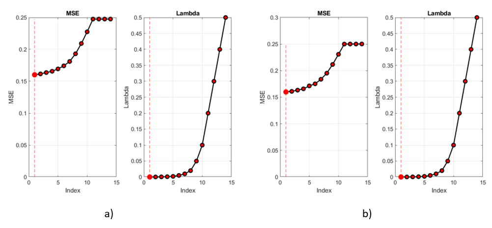
LASSO regression was used to select the most important features from these features [47]. LASSO regression is a popular regression method used to identify important features when the number of features is large. In this study, LASSO was applied to the features extracted from augmented images, with different lambda values (ranging from 0.0001 to 0.5), and feature selection was performed along with the calculation of mean squared error.
The analysis showed that the highest classification accuracy was achieved when the lambda value was 0.0001. Figure 5 shows the mean squared error values for feature selection performed using LASSO on the features extracted from augmented images.
Classification
Machine learning algorithms with various approaches were used to classify the extracted features, both collectively and separately. To give a quick explanation of these algorithms
KNN is a supervised machine learning algorithm used for classification or regression problems [48]. Predictions are made by assessing the distances between a data point and its K-nearest neighbors, with the class determined by the majority of the neighbors. In the K-Means classification, random center points are chosen, and data points are assigned to the closest center, with new center points recalculated and the data reclassified until convergence [49]. DT classify data using a branching structure where data is split based on features at each node until leaf nodes are reached [50]. A model is built using labeled input data, and new data is classified by following the branches to the appropriate leaf node for prediction.
RF is an ensemble method combining multiple decision trees, where each tree is trained on a random subset of data, and the majority vote or average of predictions is used for the result [51], [52]. The algorithm reduces overfitting and improves accuracy by selecting features from various trees and combining them to make predictions.
NB is a probabilistic classifier based on Bayes' Theorem [53], [54]. It classifies data by calculating probabilities for each class and selecting the most probable outcome. It performs well with limited training data and on imbalanced datasets.
In this study, the performance results of the classification algorithms applied to the Monkeypox dataset in Table 2 were analyzed and interpreted using metrics such as accuracy, sensitivity, specificity, precision, F1-score and AUC.
In the proposed study, features were extracted from images of the Monkeypox dataset to differentiate the disease from other types. In the study, a total of 116 features, as shown in Table 3, were obtained from images in the Monkeypox and non-Monkeypox datasets using methods such as GLCM, GLRLM, LBP, and FMOs. These features were then classified using RF, NB, KNN, and DT, and the results were analyzed.
GLCM | GLRLM | LBP | Focus Measure | Total |
22 features
| 7 features
| 59 features | 28 features
| 116 features |
The classification results for both augmented and non-augmented images, with and without SMOTE balancing, are shown in Table 4 and Table 5.
Balance | Algorithm | Accuracy | Sensitivity | Specificity | Precision | Fscore | AUC |
No | RF | 0.7243 | 0.6273 | 0.8000 | 0.7363 | 0.6700 | 0.8039 |
NB | 0.6711 | 0.6864 | 0.6571 | 0.6285 | 0.6429 | 0.7205 | |
KNN | 0.7186 | 0.6482 | 0.7776 | 0.7141 | 0.6624 | 0.7441 | |
DT | 0.6621 | 0.5873 | 0.7199 | 0.6521 | 0.6066 | 0.6885 | |
SMOTE | RF | 0.7626 | 0.7321 | 0.7936 | 0.7945 | 0.7541 | 0.8571 |
NB | 0.7222 | 0.7538 | 0.6923 | 0.7157 | 0.7256 | 0.7884 | |
KNN | 0.8137 | 0.7865 | 0.8391 | 0.8434 | 0.8029 | 0.8176 | |
DT | 0.6752 | 0.7244 | 0.6269 | 0.6742 | 0.6915 | 0.6885 |
Balance | Algorithm | Accuracy | Sensitivity | Specificity | Precision | Fscore | AUC |
No | RF | 0.8957 | 0.8543 | 0.9292 | 0.9075 | 0.8798 | 0.9553 |
NB | 0.7462 | 0.7451 | 0.7472 | 0.7061 | 0.7243 | 0.8031 | |
KNN | 0.8835 | 0.8487 | 0.9116 | 0.8862 | 0.8668 | 0.8861 | |
DT | 0.8001 | 0.7591 | 0.8334 | 0.7874 | 0.7724 | 0.8267 | |
SMOTE | RF | 0.9002 | 0.8866 | 0.9138 | 0.9115 | 0.8987 | 0.9610 |
NB | 0.7494 | 0.7846 | 0.7143 | 0.7337 | 0.7579 | 0.8043 | |
KNN | 0.8880 | 0.8884 | 0.8878 | 0.8884 | 0.8881 | 0.8924 | |
DT | 0.8056 | 0.7970 | 0.8141 | 0.8121 | 0.8038 | 0.8262 |
Table 4 presents the classification results obtained using all features with the non-augmented dataset. When SMOTE balancing was not applied, the RF algorithm achieved the highest classification performance with an accuracy of 0.7243 and an AUC value of 0.8039.
In contrast, the lowest classification performance with an accuracy of 0.6621 was shown by the DT method. When the SMOTE balancing method was applied, the best classification performance was achieved by the KNN algorithm with an accuracy of 0.8137. Additionally, the highest AUC value of 0.8571 was obtained with the RF algorithm.
In Table 5, it can be seen that without applying the SMOTE balancing method, the highest classification accuracy of 0.8957 and the highest AUC value of 0.9553 were achieved by the RF algorithm. The KNN algorithm performed close to RF with an accuracy of 0.8835 and an AUC value of 0.8861. On the other hand, the DT and NB algorithms showed relatively lower accuracy rates. When the SMOTE method was applied, the RF algorithm achieved the highest success with an accuracy of 0.9002 and an AUC value of 0.9610.
The classification algorithm performance comparison for the different feature groups (GLCM, GLRLM, LBP, and focus measures) for both imbalanced data and SMOTE balanced data is presented in Tables 6 and 7.
The classification performance with different feature groups for unbalanced data and SMOTE balanced data is presented in Table 6. In general, using SMOTE balancing improved accuracy, sensitivity, specificity, and other performance metrics significantly across all feature groups. It was found that the LBP and focus measures feature groups yielded the best performance under both conditions. The RF algorithm yielded the best results with the SMOTE balanced data for the LBP feature group (0.7420 accuracy) and the focus measures feature group (0.7417 accuracy). In addition, with the SMOTE balanced data, the KNN algorithm yielded good performance with 0.7697 accuracy under the focus measures feature group. Comparatively speaking, the GLCM and GLRLM feature groups demonstrated poorer performance than other feature groups. The results highlight the influence of different feature groups on the classification performance and the significance of the balancing method. Table 7 summarizes the classification performance with different feature groups utilizing augmented data for both unbalanced and SMOTE balanced data. In general, utilizing augmented data reported a significant increase in the overall performance of metrics. It was also ascertained that SMOTE balancing increased accuracy, sensitivity, specificity, and other metrics. The largest performance values were observed again for the focus measures and LBP feature groups.
With SMOTE-balanced data, the RF algorithm produced the best results for Focus Measures (0.8631 accuracy, 0.9357 AUC), and LBP (0.8625 accuracy, 0.9397 AUC).
The KNN algorithm performed very well for Focus Measures (0.8674 accuracy) and LBP (0.8631 accuracy) feature groups. The GLCM and GLRLM feature groups also showed good results, but slightly lower overall human performance relative to the other feature groups. The DT and NB algorithms generally produced lower performances overall; however, the application of SMOTE improved the algorithms' sensitivity and AUC scores.
The findings illustrate the positive effect of data augmentation on overall classification performance, while also highlighting the consequences of SMOTE balancing in performance success, especially when data is imbalanced.
The results of the feature selection process are presented only for those algorithms-the KNN and RF-which achieved the highest accuracy. Comparing the classification results for RF and KNN in Table 5 and Table 8 with the provided SMOTE-balanced dataset, a number of differences can be detected.
Unbalanced data | Balanced with SMOTE | ||||||||||||
|---|---|---|---|---|---|---|---|---|---|---|---|---|---|
Feature group | Algorithm | Accuracy | Sensitivity | Specificity | Precision | Fscore | AUC | Accuracy | Sensitivity | Specificity | Precision | Fscore | AUC |
GLCM | RF | 0.6579 | 0.5591 | 0.7404 | 0.6413 | 0.5901 | 0.7147 | 0.7260 | 0.7712 | 0.6808 | 0.7108 | 0.7352 | 0.8108 |
NB | 0.6409 | 0.4845 | 0.7724 | 0.6212 | 0.5209 | 0.7079 | 0.6662 | 0.6173 | 0.7154 | 0.6853 | 0.6404 | 0.7166 | |
KNN | 0.6885 | 0.5618 | 0.7923 | 0.7082 | 0.6107 | 0.7256 | 0.6709 | 0.6686 | 0.6750 | 0.6734 | 0.6642 | 0.7196 | |
DT | 0.6190 | 0.5700 | 0.6590 | 0.5874 | 0.5604 | 0.6527 | 0.6471 | 0.6205 | 0.6744 | 0.6719 | 0.6343 | 0.7140 | |
GLRLM | RF | 0.6490 | 0.5582 | 0.7224 | 0.6261 | 0.5812 | 0.6746 | 0.6665 | 0.6558 | 0.6763 | 0.6621 | 0.6473 | 0.7453 |
NB | 0.6227 | 0.6855 | 0.5699 | 0.5695 | 0.6144 | 0.6712 | 0.6197 | 0.6769 | 0.5622 | 0.6058 | 0.6381 | 0.6869 | |
KNN | 0.6507 | 0.5330 | 0.7444 | 0.6301 | 0.5674 | 0.6959 | 0.6383 | 0.5905 | 0.6867 | 0.6508 | 0.6159 | 0.7022 | |
DT | 0.6095 | 0.5727 | 0.6436 | 0.5780 | 0.5588 | 0.6472 | 0.6312 | 0.6667 | 0.5949 | 0.6307 | 0.6440 | 0.6603 | |
LBP | RF | 0.6976 | 0.6055 | 0.7692 | 0.6838 | 0.6355 | 0.7621 | 0.7420 | 0.7218 | 0.7609 | 0.7615 | 0.7355 | 0.8303 |
NB | 0.6233 | 0.7045 | 0.5564 | 0.5678 | 0.6228 | 0.7048 | 0.6232 | 0.7135 | 0.5346 | 0.6065 | 0.6488 | 0.6971 | |
KNN | 0.6401 | 0.5409 | 0.7237 | 0.6370 | 0.5709 | 0.7004 | 0.7335 | 0.7455 | 0.7212 | 0.7297 | 0.7343 | 0.7439 | |
DT | 0.6063 | 0.5727 | 0.6359 | 0.5563 | 0.5589 | 0.6353 | 0.6625 | 0.6840 | 0.6423 | 0.6630 | 0.6698 | 0.7010 | |
Focus Measures | RF | 0.7111 | 0.6327 | 0.7801 | 0.7126 | 0.6525 | 0.8074 | 0.7417 | 0.7660 | 0.7147 | 0.7335 | 0.7410 | 0.8080 |
NB | 0.6666 | 0.5382 | 0.7718 | 0.6619 | 0.5822 | 0.7109 | 0.6389 | 0.5205 | 0.7596 | 0.6869 | 0.5788 | 0.6990 | |
KNN | 0.6887 | 0.5782 | 0.7782 | 0.6881 | 0.6176 | 0.7069 | 0.7697 | 0.8179 | 0.7237 | 0.7734 | 0.7776 | 0.7708 | |
DT | 0.6310 | 0.5236 | 0.7237 | 0.6254 | 0.5438 | 0.6693 | 0.6588 | 0.5853 | 0.7276 | 0.7034 | 0.6287 | 0.6924 | |
Unbalanced data | Balanced with SMOTE | ||||||||||||
|---|---|---|---|---|---|---|---|---|---|---|---|---|---|
Feature group | Algorithm | Accuracy | Sensitivity | Specificity | Precision | Fscore | AUC | Accuracy | Sensitivity | Specificity | Precision | Fscore | AUC |
GLCM | RF | 0.8139 | 0.7423 | 0.8719 | 0.8248 | 0.7811 | 0.8862 | 0.8257 | 0.8005 | 0.8509 | 0.8436 | 0.8210 | 0.9011 |
NB | 0.7168 | 0.6807 | 0.7461 | 0.6849 | 0.6824 | 0.7586 | 0.7112 | 0.7035 | 0.7189 | 0.7147 | 0.7088 | 0.7605 | |
KNN | 0.8180 | 0.7892 | 0.8413 | 0.8028 | 0.7952 | 0.8152 | 0.8370 | 0.8395 | 0.8345 | 0.8356 | 0.8369 | 0.8427 | |
DT | 0.7569 | 0.7059 | 0.7982 | 0.7387 | 0.7210 | 0.7892 | 0.7528 | 0.7585 | 0.7472 | 0.7501 | 0.7541 | 0.7847 | |
GLRLM | RF | 0.8008 | 0.7304 | 0.8577 | 0.8072 | 0.7659 | 0.8727 | 0.8183 | 0.7965 | 0.8401 | 0.8345 | 0.8145 | 0.8888 |
NB | 0.6613 | 0.6807 | 0.6457 | 0.6102 | 0.6422 | 0.7232 | 0.6590 | 0.7228 | 0.5952 | 0.6413 | 0.6791 | 0.7160 | |
KNN | 0.7809 | 0.7363 | 0.8167 | 0.7646 | 0.7495 | 0.7765 | 0.8100 | 0.8068 | 0.8132 | 0.8120 | 0.8093 | 0.8100 | |
DT | 0.7384 | 0.6974 | 0.7715 | 0.7123 | 0.7039 | 0.7644 | 0.7545 | 0.7335 | 0.7755 | 0.7665 | 0.7490 | 0.7862 | |
LBP | RF | 0.8456 | 0.8109 | 0.8736 | 0.8388 | 0.8245 | 0.9256 | 0.8625 | 0.8685 | 0.8566 | 0.8587 | 0.8632 | 0.9397 |
NB | 0.6764 | 0.6695 | 0.6819 | 0.6308 | 0.6489 | 0.7483 | 0.6876 | 0.7126 | 0.6627 | 0.6793 | 0.6951 | 0.7633 | |
KNN | 0.8293 | 0.8025 | 0.8509 | 0.8140 | 0.8079 | 0.8267 | 0.8631 | 0.8815 | 0.8447 | 0.8504 | 0.8656 | 0.8631 | |
DT | 0.7469 | 0.6933 | 0.7902 | 0.7293 | 0.7099 | 0.7737 | 0.7687 | 0.7716 | 0.7659 | 0.7675 | 0.7693 | 0.7918 | |
Focus Measures | RF | 0.8549 | 0.8110 | 0.8905 | 0.8587 | 0.8335 | 0.9317 | 0.8631 | 0.8498 | 0.8765 | 0.8739 | 0.8612 | 0.9357 |
NB | 0.6945 | 0.6975 | 0.6921 | 0.6480 | 0.6715 | 0.7436 | 0.7001 | 0.7466 | 0.6537 | 0.6840 | 0.7135 | 0.7566 | |
KNN | 0.8377 | 0.7969 | 0.8708 | 0.8335 | 0.8145 | 0.8458 | 0.8674 | 0.8622 | 0.8725 | 0.8721 | 0.8669 | 0.8748 | |
DT | 0.7986 | 0.7675 | 0.8237 | 0.7792 | 0.7731 | 0.8272 | 0.7905 | 0.7772 | 0.8039 | 0.8005 | 0.7878 | 0.8239 | |
In the case of RF, the provided data without feature selection performs better in terms of accuracy (0.9002 vs. 0.8974), sensitivity (0.8866 vs. 0.8792), and F-score (0.8987 vs. 0.8954). On the other hand, Table 5 shows a marginally higher specificity of 0.9155 versus 0.9138 and precision of 0.9126 versus 0.9115. The AUC values for RF are almost identical, standing at 0.9611 in Table 5 and 0.9610 in the provided data, which means that the overall capability of classification would be similar. As for KNN, Table 5 shows slightly better performance in nearly all metrics like accuracy at 0.8914 versus 0.8880, sensitivity at 0.8923 versus 0.8884, specificity at 0.8906 versus 0.8878, F-score at 0.8915 versus 0.8881, and AUC at 0.8924 versus 0.8982. The precision is also nearly identical in both datasets, standing at 0.8914 in Table 8 and 0.8884 in the provided data.
While RF does a little better with the data provided, KNN largely performed marginally higher in Table 5, however, noted the differences were small. The purpose of these comparisons was to show the influence that feature selection and processing has on classification performance. These comparisons give effect to performance differences across the various datasets and indicate that while RF noticeably receives most of its benefits from pre-processing and feature selection for the data presented, KNN was improved performance in Table 5. While feature selection often improves model performance by characteristically reducing noise and irrelevant data, in the case where all the feature are managed without overfitting like RF, reducing features could result in lower classification performance.
Reducing features for KNN is beneficial as it reduces the dimensionality of the feature space, enhances the distance metric relevance, and provides KNN with greater capacity to discriminate between classes. Therefore KNN becomes a method that can derive benefit from Lasso feature selection.
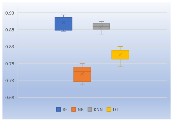
In Figure 6, the accuracy values of different algorithms (RF, NB, KNN, and DT) are plotted as boxplots, for each fold on the SMOTE balanced dataset. It illustrates the classification performance along with accuracy's distribution enabling comparison of the four algorithms and their variations in accuracy. The RF algorithm produced the best accuracy performance through and average accuracy of 0.9002. Additionally, the narrow distribution of RF's boxplot shows it produced more steady accuracy values over each of the folds, indicative of a more stable algorithm. The K Nearest Neighbors (KNN) algorithm performed analogously well to RF, produced a similar narrow distribution and resulted in a slightly lower performance accuracy of 0.8880. The Decision Tree (DT) had a significantly lower average classification performance of approximately 0.8056. Associated with this lower performance, a wider range of accuracy values was noticed with this algorithm further evidenced through the variable performance in folds. NB produced the lowest accuracy as compared to the other three algorithms, with an approximate average accuracy of 0.75, and is supported with the additional observation of having the highest amount of variance compared to the other three algorithms.
On the whole, RF and KNN performed best in classifying the instances in the SMOTE-balanced dataset, while DT, and especially NB, had poor performance. The high accuracy and consistency obtained by RF make it the most reliable algorithm for this dataset.
This research differs significantly in terms of the methods employed and the characteristics examined in contrast to existing methods for classifying monkeypox disease. Ali et al. [19] aimed to perform direct image classification using deep learning-based models and our proposed study aimed to investigate traditional machine learning algorithms and various feature extraction methods in order to determine the most effective combinations. In [19], the researchers used deep learning models that had been pre-trained such as ResNet50, VGG-16, and InceptionV3, to automatically classify monkeypox and other diseases. They created an ensemble model, but the best accuracy was reached using the ResNet50 model which achieved an 82.96% accuracy rate. The authors acknowledged that their dataset was limited and emphasized the need for a broader and more diverse dataset. In our proposed study, we experimented with data that had been captured using the different feature extraction methods compared such as GLCM, GLRLM, LBP, and Focus Measures by traditional machine learning algorithms such as RF, KNN, NB, and DT. In addition, this study examines the ways data augmentation and SMOTE balancing methods impact classification performance. The RF model performed the best in this study with a 90.02% accuracy rate and 96.10% AUC score.
A study by Yasmin et al. [30] used a deep learning-based approach for diagnosing monkeypox disease. Using transfer learning, six different deep learning models were trained, and the model with the best performance was fine-tuned to create the PoxNet22 model, which achieved 100% accuracy, sensitivity, and precision. While our proposed study achieved lower accuracy rates than deep learning methods, it demonstrates that the model provides a balanced and generalizable structure with smaller datasets.
This research shows that using data augmentation, balanced datasets, and appropriate feature extraction methods can significantly improve the classification of monkeypox disease through images. When all feature groups were assessed, the LBP and Focus Measures gave the highest classification performance, especially with the random forest and k-nearest neighbor learning algorithms. SMOTE also improved classification accuracy, sensitivity, and AUC for most models. The use of SMOTE indicates the need to address imbalance in classification tasks. In general, the RF algorithm provided the best performance at 90.02% accuracy and 96.10% AUC when applied to the augmented dataset. The present study demonstrates the potential for machine learning-based approaches to accurately detect monkeypox disease. Future work should aim to expand the dataset, incorporate additional feature groups, and assess the hybrid or pure deep learning models to further builds upon generalizability and performance.
References
- 1.[1] A. M. McCollum and I. K. Damon, “Human monkeypox,” Clin. Infect. Dis., vol. 58, no. 2, pp. 260–267, 2014.
- 2.[2] L. D. Bethineedi, L. V. S. Kutikuppala, and V. Kandi, “Monkeypox epidemic: a throwback from smallpox eradication,” Cureus, vol. 14, no. 7, 2022.
- 3.[3] B. Moss, “Poxvirus DNA replication,” Cold Spring Harb. Perspect. Biol., vol. 5, no. 9, p. a010199, 2013.
- 4.[4] M. Pal, F. Mengstie, and V. Kandi, “Epidemiology, diagnosis, and control of monkeypox disease: a comprehensive review,” Am J Infect Dis Microbiol, vol. 5, no. 2, pp. 94–99, 2017.
- 5.[5] A. K. Rao, “Use of JYNNEOS (smallpox and monkeypox vaccine, live, nonreplicating) for preexposure vaccination of persons at risk for occupational exposure to orthopoxviruses: recommendations of the Advisory Committee on Immunization Practices—United States, 2022,” MMWR. Morb. Mortal. Wkly. Rep., vol. 71, 2022.
- 6.[6] A. W. Rimoin et al., “Major increase in human monkeypox incidence 30 years after smallpox vaccination campaigns cease in the Democratic Republic of Congo,” Proc. Natl. Acad. Sci., vol. 107, no. 37, pp. 16262–16267, 2010.
- 7.[7] P. von Magnus, E. K. Andersen, K. B. Petersen, and A. Birch Andersen, “A pox-like disease in cynomolgus monkeys.,” 1959.
- 8.[8] J. G. Breman, M. V Steniowski, E. Zanotto, A. I. Gromyko, and I. Arita, “Human monkeypox, 1970-79,” Bull. World Health Organ., vol. 58, no. 2, p. 165, 1980.
- 9.[9] J. P. Thornhill et al., “Monkeypox virus infection in humans across 16 countries—April–June 2022,” N. Engl. J. Med., vol. 387, no. 8, pp. 679–691, 2022.
- 10.[10] W. H. Organization, “Monkeypox https://www. who. int/news-room/fact-sheets/detail/monkeypox,” Accessed 10th Jun, 2022.
- 11.[11] F. B. Demir et al., “MNPDenseNet: automated monkeypox detection using multiple nested patch division and pretrained densenet201,” Multimed. Tools Appl., pp. 1–23, 2024.
- 12.[12] D. Uzun Ozsahin, M. T. Mustapha, B. Uzun, B. Duwa, and I. Ozsahin, “Computer-aided detection and classification of monkeypox and chickenpox lesion in human subjects using deep learning framework,” Diagnostics, vol. 13, no. 2, p. 292, 2023.
- 13.[13] O. C. Abanobi, “Factors associated with the practice of monkey pox preventive behaviours among health workers in Yenagoa LGA, Bayelsa state, Nigeria”.
- 14.[14] N. Fatima and K. Mandava, “Monkeypox-a menacing challenge or an endemic?,” Ann. Med. Surg., vol. 79, p. 103979, 2022.
- 15.[15] A. S. Jaradat et al., “Automated monkeypox skin lesion detection using deep learning and transfer learning techniques,” Int. J. Environ. Res. Public Health, vol. 20, no. 5, p. 4422, 2023.
- 16.[16] M. M. Ahsan, M. R. Uddin, M. Farjana, A. N. Sakib, K. Al Momin, and S. A. Luna, “Image Data collection and implementation of deep learning-based model in detecting Monkeypox disease using modified VGG16,” arXiv Prepr. arXiv2206.01862, 2022.
- 17.[17] M. Manjurul Ahsan, M. Ramiz Uddin, and S. Akter Luna, “Monkeypox Image Data collection,” arXiv e-prints, p. arXiv-2206, 2022.
- 18.[18] C. Sitaula and T. B. Shahi, “Monkeypox virus detection using pre-trained deep learning-based approaches,” J. Med. Syst., vol. 46, no. 11, p. 78, 2022.
- 19.[19] S. N. Ali et al., “Monkeypox skin lesion detection using deep learning models: A feasibility study,” arXiv Prepr. arXiv2207.03342, 2022.
- 20.[20] M. A. Hussain, T. Islam, F. U. H. Chowdhury, and B. M. R. Islam, “Can artificial intelligence detect Monkeypox from digital skin images?,” BioRxiv, pp. 2008–2022, 2022.
- 21.[21] V. H. Sahin, I. Oztel, and G. Yolcu Oztel, “Human monkeypox classification from skin lesion images with deep pre-trained network using mobile application,” J. Med. Syst., vol. 46, no. 11, p. 79, 2022.
- 22.[22] D. J. Matuszewski and I.-M. Sintorn, “TEM virus images: Benchmark dataset and deep learning classification,” Comput. Methods Programs Biomed., vol. 209, p. 106318, 2021.
- 23.[23] A. A. Abdelhamid et al., “Classification of monkeypox images based on transfer learning and the Al-Biruni Earth Radius Optimization algorithm,” Mathematics, vol. 10, no. 19, p. 3614, 2022.
- 24.[24] U. Singh and L. S. Songare, “Analysis and detection of monkeypox using the GoogLeNet Model,” in 2022 International Conference on Automation, Computing and Renewable Systems (ICACRS), IEEE, 2022, pp. 1000–1008.
- 25.[25] M. Dwivedi, R. G. Tiwari, and N. Ujjwal, “Deep learning methods for early detection of monkeypox skin lesion,” in 2022 8th International Conference on Signal Processing and Communication (ICSC), IEEE, 2022, pp. 343–348.
- 26.[26] V. Kumar, “Analysis of CNN features with multiple machine learning classifiers in diagnosis of monkeypox from digital skin images,” MedRxiv, pp. 2009–2022, 2022.
- 27.[27] A. I. Saleh and A. H. Rabie, “Human monkeypox diagnose (HMD) strategy based on data mining and artificial intelligence techniques,” Comput. Biol. Med., vol. 152, p. 106383, 2023.
- 28.[28] S. Bengesi, T. Oladunni, R. Olusegun, and H. Audu, “A machine learning-sentiment analysis on monkeypox outbreak: An extensive dataset to show the polarity of public opinion from Twitter tweets,” IEEE Access, vol. 11, pp. 11811–11826, 2023.
- 29.[29] D. Bala et al., “MonkeyNet: A robust deep convolutional neural network for monkeypox disease detection and classification,” Neural Networks, vol. 161, pp. 757–775, 2023.
- 30.[30] F. Yasmin et al., “PoxNet22: A fine-tuned model for the classification of monkeypox disease using transfer learning,” Ieee Access, vol. 11, pp. 24053–24076, 2023.
- 31.[31] N. V Chawla, K. W. Bowyer, L. O. Hall, and W. P. Kegelmeyer, “SMOTE: synthetic minority over-sampling technique,” J. Artif. Intell. Res., vol. 16, pp. 321–357, 2002.
- 32.[32] M. Yavaş, A. Güran, and M. Uysal, “Covid-19 veri kümesinin SMOTE tabanlı örnekleme yöntemi uygulanarak sınıflandırılması,” Avrupa Bilim ve Teknol. Derg., pp. 258–264, 2020.
- 33.[33] R. HEPHZIBAH, A. H. CHRISTINAL, D. M. ALEX, R. JAYANTHI, D. A. CHANDY, and C. BAJAJ, “A hybrid model of random forest ensemble and resample for cardiotocography data classification.,” Sigma J. Eng. Nat. Sci. ve Fen Bilim. Derg., vol. 43, no. 2, 2025.
- 34.[34] T. Subramaniam, H. A. Jalab, R. W. Ibrahim, and N. F. Mohd Noor, “Improved image splicing forgery detection by combination of conformable focus measures and focus measure operators applied on obtained redundant discrete wavelet transform coefficients,” Symmetry (Basel)., vol. 11, no. 11, p. 1392, 2019.
- 35.[35] S. Pertuz, D. Puig, and M. A. Garcia, “Analysis of focus measure operators for shape-from-focus,” Pattern Recognit., vol. 46, no. 5, pp. 1415–1432, 2013.
- 36.[36] R. M. Haralick, K. Shanmugam, and I. H. Dinstein, “Textural features for image classification,” IEEE Trans. Syst. Man. Cybern., no. 6, pp. 610–621, 1973.
- 37.[37] A. Çalışkan, E. Acar, and Y. Kaya, “GLCM TABANLI K-NN SINIFLANDIRICI MODELİ İLE AVUÇ İÇİ TANIMA SİSTEMİ,” Batman Üniversitesi Yaşam Bilim. Derg., vol. 1, no. 2, pp. 1–10, 2012.
- 38.[38] K. Gajalakshmi and S. Saravanan, “Automatic identification of brittle, elongated and equiaxed ductile fracture modes in weld joints through machine learning.,” Sigma J. Eng. Nat. Sci. ve Fen Bilim. Derg., vol. 43, no. 2, 2025.
- 39.[39] S. S. Sastry, T. V. Kumari, C. N. Rao, K. Mallika, S. Lakshminarayana, and H. S. Tiong, “Transition temperatures of thermotropic liquid crystals from the local binary gray level cooccurrence matrix,” Adv. Condens. Matter Phys., vol. 2012, no. 1, p. 527065, 2012.
- 40.[40] Ş. Öztürk and B. Akdemir, “Application of feature extraction and classification methods for histopathological image using GLCM, LBP, LBGLCM, GLRLM and SFTA,” Procedia Comput. Sci., vol. 132, pp. 40–46, 2018.
- 41.[41] F. Albregtsen, B. Nielsen, and H. E. Danielsen, “Adaptive gray level run length features from class distance matrices,” in Proceedings 15th International Conference on Pattern Recognition. ICPR-2000, IEEE, 2000, pp. 738–741.
- 42.[42] A. K. Mohanty, S. Beberta, and S. K. Lenka, “Classifying benign and malignant mass using GLCM and GLRLM based texture features from mammogram,” Int. J. Eng. Res. Appl., vol. 1, no. 3, pp. 687–693, 2011.
- 43.[43] V. Durgamahanthi, J. Anita Christaline, and A. Shirly Edward, “GLCM and GLRLM based texture analysis: application to brain cancer diagnosis using histopathology images,” in Intelligent Computing and Applications: Proceedings of ICICA 2019, Springer, 2021, pp. 691–706.
- 44.[44] A. Gunay and V. V Nabiyev, “Automatic age classification with LBP,” in 2008 23rd international symposium on computer and information sciences, IEEE, 2008, pp. 1–4.
- 45.[45] M. Heikkilä, M. Pietikäinen, and C. Schmid, “Description of interest regions with local binary patterns,” Pattern Recognit., vol. 42, no. 3, pp. 425–436, 2009.
- 46.[46] T. Şentürk et al., “Histopathological Image Analysis Using Machine Learning to Evaluate Cisplatin and Exosome Effects on Ovarian Tissue in Cancer Patients,” Appl. Sci., vol. 15, no. 4, p. 1984, 2025.
- 47.[47] R. Muthukrishnan and R. Rohini, “LASSO: A feature selection technique in predictive modeling for machine learning,” in 2016 IEEE international conference on advances in computer applications (ICACA), Ieee, 2016, pp. 18–20.
- 48.[48] M. Suyal and P. Goyal, “A review on analysis of K-nearest neighbor classification machine learning algorithms based on supervised learning,” Int. J. Eng. Trends Technol., vol. 70, no. 7, pp. 43–48, 2022.
- 49.[49] H. Demir, P. Erdoğmuş, and M. Kekeçoğlu, “Destek Vektör Makineleri, YSA, K-Means ve KNN Kullanarak Arı Türlerinin Sınıflandırılması,” Düzce Üniversitesi Bilim ve Teknol. Derg., vol. 6, no. 1, pp. 47–67, 2018.
- 50.[50] A. Nafees et al., “Forecasting the mechanical properties of plastic concrete employing experimental data using machine learning algorithms: DT, MLPNN, SVM, and RF,” Polymers (Basel)., vol. 14, no. 8, p. 1583, 2022.
- 51.[51] P. Dinesh, A. S. Vickram, and P. Kalyanasundaram, “Medical image prediction for diagnosis of breast cancer disease comparing the machine learning algorithms: SVM, KNN, logistic regression, random forest and decision tree to measure accuracy,” in AIP Conference Proceedings, AIP Publishing, 2024.
- 52.[52] B. Daş and İ. Türkoğlu, “DNA dizilimlerinin sınıflandırılmasında karar ağacı algoritmalarının karşılaştırılması,” 2014.
- 53.[53] H. T. Zaw, N. Maneerat, and K. Y. Win, “Brain tumor detection based on Naïve Bayes Classification,” in 2019 5th International Conference on engineering, applied sciences and technology (ICEAST), IEEE, 2019, pp. 1–4.
- 54.[54] T. Özcan, “Yığınlanmış özdevinimli kodlayıcılar ile göğüs kanserinin sınıflandırılması ve klasik makine öğrenme metotları ile performans karşılaştırması,” Erciyes Üniversitesi Fen Bilim. Enstitüsü Fen Bilim. Derg., vol. 36, no. 2, pp. 151–160, 2020.