Abstract
EEG signals can be used to accurately classify stress levels using machine learning techniques and a limited number of brain channels.
Researchers used the Empirical Wavelet Transform to break down EEG signals into smaller parts and then applied machine learning algorithms to classify stress levels. They found that using a Random Forest classifier with a limited number of EEG channels was effective in identifying stress levels, with an accuracy of 86.25% for binary classification. The most useful features for classification were related to signal power, relative energy, and amplitude, particularly from frontal and temporal brain channels.
Full TextOpen Access
Recently, there has been a growing interest in identifying and classifying the level of stress experienced by a person when they are engaged in everyday activities or performing tasks, such as examinations, through electroencephalography (EEG) signals [1]. Numerous advancements in signal processing analysis techniques have raised interest towards stress assessment using EEG signals.
Classification studies based on machine learning and deep learning techniques have also been employed on the extracted EEG feature sets within several research works. Hybrid models that use time domain and frequency domain feature sets combined with machine learning classification tools are commonly utilized for stress detection [1–3]. Recent studies have shown that hybrid approaches provide promising outcomes in distinguishing between different stress states. Review studies focusing on EEG-based mental stress assessment underline the importance of understanding the underlying neural mechanisms associated with stress. In this context, spatial patterns in EEG signals are often analyzed using convolution-based structures, while temporal variations are examined through sequence-oriented models. Combining spatial and temporal representations allows a more detailed characterization of the complex and time-varying nature of EEG signals related to mental stress, leading to more reliable stress assessment outcomes [4].
To further enhance stress detection performance, hybrid frameworks incorporating signal processing and learning-based approaches have been widely explored. In several studies, EEG signals are first decomposed using time–frequency techniques to suppress noise and highlight relevant components, followed by automated feature learning for classification. Different sequential modeling strategies have been employed to capture temporal dependencies within EEG recordings, resulting in improved discrimination between stress levels compared to conventional approaches. In addition to model design, EEG channel selection has been identified as a critical factor in stress analysis. Methods based on statistical relationships between signal characteristics have demonstrated that frontal brain regions are particularly sensitive to mental stress, emphasizing their relevance for practical and wearable stress monitoring systems [5,6].
Additionally, the significance of certain frequency bands in the analysis of stress, especially alpha and beta waves, has been highlighted in some related studies. As reflected in some sources, the alpha band is dominantly active during states of relaxation or lack of stress, while the beta band becomes relatively active during stress, especially while taking certain examination types [1,7]. Most related studies have been focused on the prefrontal area of the brain, as the prefrontal region of the brain is known to be significantly involved in cognitive processing, as well as in the regulation of emotions. Therefore, prefrontal EEG brain signals have been observed to be highly informative in assessing the mental state of the individual [1].
EEG-based detection of stress has been limited by the nature of EEG signals as random, non-stationary, nonlinear, and often weakly-correlated with each other. In order to obtain or extract emotion-related or stress-relevant information from such a complex set of signals, sophisticated signal processing methods must be used. Furthermore, many of the studies that have been conducted in the past have been based on either one domain (e.g. only the time domain) or on a single analysis method, limiting the number of fundamental features that can be identified. As a result, it can be difficult to reliably differentiate among various levels of stress. Therefore, in this study, stress levels experienced during exams are classified as low, moderate, and high stress levels using time-domain and frequency-domain features extracted from a limited number of EEG channels. Both binary and multi-class classification frameworks are employed to evaluate the effectiveness of the proposed approach, with the aim of achieving reliable stress assessment while reducing system complexity and computational cost.
Dataset and preprocessing
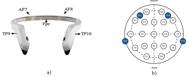
In this study, open-access EEG signals collected from students during an exam were recorded using a Muse 2 EEG headband at a sampling frequency of 256 Hz [8]. The signals were recorded as 4 channels (TP9, AF7, AF8, TP10) as shown in Figure 1, including both raw signals and EEG subbands (Delta, Theta, Alpha, Beta, and Gamma). Recordings were taken throughout the exam and include timestamps and motion information. EEG signals were generally obtained in a short period of time, less than 5 minutes. The EEG subbands are processed and the data is normalized. However, in this study, only the raw EEG data from the four channels were analyzed. 26 participants (19 women, 7 men; mean age: 21.23 ± 1.14) participated in the study. Detailed information about the participants is given in Table 1.
During preprocessing, missing values in the signals were identified and removed prior to feature extraction. The data was then filtered using a fourth-order Butterworth filter, a [0.5 Hz - 30 Hz] band-pass filter, and a 50 Hz IIR notch filter, before being separated into four subbands using the Empirical Wavelet Transform (EWT) method. The features were extracted from four separate EWT subbands corresponding to four EEG channels.
Stress Level | Number of participants | Gender | Age | Stress score | |
|
| Female | Male | Mean+SD | Mean+SD |
low | 8 | 4 | 4 | 20.63 ± 0.82 | 3.75 ± 1.83 |
moderate | 8 | 6 | 2 | 22.13 ± 1.13 | 10.63 ± 2.62 |
high | 10 | 9 | 1 | 21.00 ± 0.94 | 17.80 ± 2.35 |
Total | 26 | 19 | 7 | 21.23 ± 1.14 | 11.27 ± 6.33 |
Empirical Wavelet Transform
In this study, EEG signals were first decomposed using the Empirical Wavelet Transform (EWT) prior to feature extraction. Although decomposition techniques such as EMD and VMD have been widely used in the literature, they suffer from limitations including high computational cost, mode mixing, and methodological complexity. Introduced by Gilles [9] in 2013, EWT is an adaptive time–frequency analysis method that constructs signal-specific wavelets by segmenting the Fourier spectrum into meaningful frequency bands as seen in Equation (1). Multiresolution signal decomposition that more accurately captures the inherent properties of EEG signals is made possible by this adaptive structure [9]. The input signal (in the time domain) is represented by x in Equation (1), and the scaling and wavelet functions are denoted by φ and ρ, respectively.
After preprocessing the EEG signals, they were decomposed into 4 EWT subbands, and the features were extracted from these subband signals.
$W_x^d (n,t)=⟨x┤,├ φ_n ⟩=∫▒〖x(τ)(φ_n (τ-t)) ̅ 〗 dτ=(x ̂(ω)(φ_n (ω)) ̅ )^v$
Feature Extraction
In this study, various features from both the time domain and the frequency domain were extracted to classify stress levels. Time-domain features were extracted to characterize the statistical and dynamical properties of the normalized signal, including signal power, skewness, kurtosis, mean absolute amplitude, Teager–Kaiser energy, autoregressive (AR) model coefficients, zero-crossing rate, Lyapunov exponent, total harmonic distortion, Katz fractal dimension, and the Hurst exponent. In addition, frequency-domain features were computed using the Power Spectral Density (PSD) estimated via Welch’s method. These features include peak frequency and power, spectral power statistics (mean, variance, skewness, and kurtosis), energy-based ratios, total and relative spectral energy, and spectral entropy, which collectively describe the spectral distribution and complexity of the signal. Table 2 contains brief descriptions of the features.
The frequency-domain features extracted in this study have previously been applied to EEG signals and shown to yield successful results [10]. Similarly, in another study, comparable time-domain features were derived from EEG recordings, demonstrating promising performance [11]. Detailed mathematical formulations of the extracted features can be found in references [10] and [11]. In total, 30 features were extracted from each EWT subband. Since there are 4 EEG channels, a total of 120 features were obtained.
The primary motivation for selecting these features was to evaluate stress level classification performance using computationally efficient and easily interpretable signal characteristics. Instead of relying on complex and time-consuming measures such as advanced entropy-based features, a set of simple time- and frequency-domain features was employed to assess whether reliable stress discrimination can be achieved with reduced computational cost.
No | Feature Name | Description |
1 | Power | Mean squared value of the normalized signal (signal power for time domain) |
2 | Skewness | Measure of asymmetry of the signal amplitude distribution |
3 | Kurtosis | Measure of the peakedness of the signal amplitude distribution |
4 | MeanAmp | Mean absolute value of the signal amplitude |
5 | TKE | Mean Teager–Kaiser energy of the signal |
6-9 | AR Coefficients (AR1–AR4) | Autoregressive model coefficients of order 4 using Yule-Walker method (representing short-term signal dynamics) |
10 | ZCR | Zero-crossing rate of the signal |
11 | Lyap | Lyapunov exponent indicating chaotic behavior |
12 | THD | Total harmonic distortion of the signal |
13 | KFD | Katz fractal dimension measuring signal complexity |
14 | Hurst | Hurst exponent obtained via Detrended Fluctuation Analysis (DFA) |
15 | TotalPSD | Total PSD; see Eq. (3) |
16 | RelEnergy | Relative spectral energy normalized by signal power |
17 | SpecEntropy | Spectral entropy of the normalized PSD |
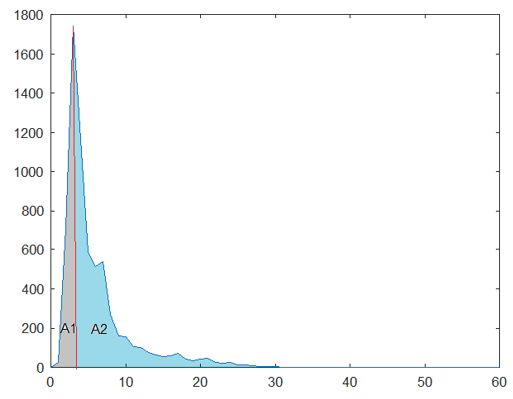
18 | AUC1 | Area under the PSD curve up to the peak power (A1); see Fig. 2 |
19 | AUC2 | Area under the PSD curve after the peak power (A2); see Fig. 2 |
20 | Rate1 | Ratio A1 / (A1 + A2) |
21 | Rate2 | Ratio A1 / A2 |
22 | Rate3 | Ratio A2 / (A1 + A2) |
23 | Maxf | Frequency corresponding to the maximum PSD value |
24 | Maxp | Maximum power value of the PSD |
25 | Minp | Minimum power value of the PSD |
26 | Diffp | Difference between maximum and minimum PSD power |
27 | MeanPSD | Mean value of the PSD |
28 | StdPSD | Standard deviation of the PSD |
29 | KurtPSD | Kurtosis of the PSD distribution |
30 | SkewPSD | Skewness of the PSD distribution |
Statistical Analysis
Following the extraction of features from the EEG recordings corresponding to different stress levels, statistical analyses were conducted to investigate group-wise differences. R Statistics (R Studio software, version R-4.4.2) was used for statistical testing in accordance with standard procedure in the literature for multi-group comparisons. To determine if the feature distributions were normal at a significance level of p = 0.05, the Kolmogorov–Smirnov test was initially used. Non-parametric statistical analysis was used when at least one stress group did not meet the normalcy assumption. Thus, the association between stress levels and the retrieved EEG features was assessed using the Kruskal-Wallis (non-parametric) and ANOVA (parametric) tests. Pairwise comparisons between the stress groups were conducted using either the Tukey test or Dunn's post hoc test when statistically significant differences were found.
Data Balancing with SMOTE
In the study, 8 individuals were assigned to the low-stress level group, 8 to the moderate-stress level group, and 10 to the high-stress level group. When the EWT was divided into subbands, the EEG signal comprised 4 subbands, resulting in 32 samples for low stress, 32 samples for moderate stress, and 40 samples for high stress. To balance the sample size between the classes, the Synthetic Minority Oversampling Technique (SMOTE) method [12,13] was applied, and the number of samples was equalized to 40 for all stress levels. This aimed to reduce bias in groups with a large sample size.
Machine Learning Models
In this study, classification algorithms with different methodologies were used: K-nearest neighbor (K-NN), Support Vector Machine (SVM), Artificial Neural Network (ANN), Random Forest (RF), and Adaptive Boost (AdaBoost). To improve model performance and reduce overfitting, the algorithms' hyperparameters were tuned using Bayesian optimization.
The KNN algorithm is a non-parametric, instance-based learning method used for classification and regression, where decision making is deferred until classification [14]. In KNN, an unlabeled sample is assigned to the class most frequently represented among its K nearest neighbors, which are determined based on a distance metric [14]. The SVM is a powerful supervised learning algorithm that constructs an optimal decision hyperplane by maximizing the margin between classes [15]. For nonlinearly separable data, SVM employs kernel functions to map the data into a higher-dimensional feature space, enabling effective classification [15]. ANN is a computational model inspired by the structure of the human brain, consisting of interconnected neurons organized in layers [16]. By adjusting connection weights through a learning process, ANNs are capable of modeling complex nonlinear relationships for classification and prediction tasks [16]. RF improves prediction stability while decreasing variance, making it ideal for complicated and heterogeneous datasets like those found in medical research [17]. The AdaBoost algorithm creates an ensemble of weak classifiers (most typically decision trees) by weighting each one based on its classification accuracy. AdaBoost prioritizes misclassified examples in an iterative process of training and updating sample weights, allowing the ensemble to learn complex decision boundaries [17,18].
| Predicted Class | |||
Low stress level | Moderate stress level | High stress level | ||
Actual Class | Low stress level | TP | FN | FN |
Moderate stress level | FP | TN | TN | |
High stress level | FP | TN | TN | |
Statistical Analysis Results
Table 4 presents only the features that showed significant differences (p<0.05) between groups (stress levels) and their p-values. According to the statistical analysis results, significant differences were observed predominantly in the AF7 EEG channel. In this channel, statistically significant differences were found in stress levels for power, mean amplitude (MeanAmp), total power spectral density (TotalPSD), relative energy (RelEnergy), mean and standard deviation power values (MeanPSD, StdPSD), and parameters related to maximum and minimum power (p < 0.05). Furthermore, temporal-energy based (TKE) and fractal dimension (KFD) features also showed significant discrimination in the AF7 channel. In addition, a significant difference was detected only for the Maxf feature in the TP10 channel (p = 0.0441), while no significant differences were observed in the TP9 and AF8 channels in terms of the analyzed features.
These findings demonstrate that stress levels have a significant impact on both the energy-based and complexity/fractal features of the EEG signal, particularly in the AF7 channel corresponding to the frontal region. The significant findings of numerous features in the AF7 channel support a strong correlation between stress and prefrontal cortex activity. In contrast, the lack of significant results in the TP9 and AF8 channels suggests that stress-related EEG changes are channel-dependent and regional. The fact that only one feature was significant in the TP10 channel suggests that this region offers a limited but complementary contribution to stress discrimination.
EEG Channel | Power | MeanAmp | TKE | KFD | TotalPSD | RelEnergy | AUC1 | AUC2 | Maxf | Maxp | Minp | Diffp | MeanPSD | StdPSD |
TP9 |
|
|
|
|
|
|
|
|
|
|
|
|
|
|
AF7 | 0.0040 | 0.0025 | 0.0281 | 0.0230 | 0.0044 | 0.0014 | 0.0038 | 0.0384 |
| 0.0039 | 0.0088 | 0.0039 | 0.0039 | 0.0042 |
AF8 |
|
|
|
|
|
|
|
|
|
|
|
|
|
|
TP10 |
|
|
|
|
|
|
|
| 0.0441 |
|
|
|
|
|
The results given in Table 5 are the post-hoc analysis results of the second EEG channel (AF7). Statistical significance is denoted as p < 0.05 (***), p < 0.01 (**), and p < 0.001 ( *** ). A dash (–) indicates no statistically significant difference. The post-hoc analysis results presented in Table 5 show that differences in stress levels in the AF7 channel are particularly pronounced in the low-high stress comparison. Strong and significant differences were observed between low and high stress levels in most statistical measures related to power, mean amplitude (MeanAmp), total power spectral density (TotalPSD), relative energy (RelEnergy), and power distribution (p < 0.01 and p < 0.001).
In contrast, no significant differences were found for any feature in the moderate-high stress levels comparisons. Between low and moderate stress levels, only limited significance was found in some energy and amplitude-based features. These results indicate that EEG features in the AF7 channel change gradually as the stress level increases, and that high stress conditions, in particular, produce a more distinctive physiological response compared to low stress level.
Feature Name | Low–Moderate | Low–High | Moderate–High |
Power | * | ** | – |
MeanAmp | * | ** | – |
TKE | – | * | – |
KFD | – | * | – |
TotalPSD | * | ** | – |
RelEnergy | ** | ** | – |
AUC1 | * | ** | – |
AUC2 | – | * | – |
Maxp | * | ** | – |
Minp | – | ** | – |
Diffp | * | ** | – |
MeanPSD | * | ** | – |
StdPSD | * | ** | – |
Classification Results
In this study, MATLAB software was used for preprocessing, feature extraction, and classification, while WEKA software was used for data balancing and feature selection. Feature selection was performed using the Correlation-based Feature Subset Evaluator (CfsSubsetEval) with BestFirst search, which selects feature subsets that are highly correlated with the class labels while minimizing inter-feature redundancy. The classification procedures were carried out for both binary and multiclass scenarios. A total of 30 features were extracted from each EEG channel, resulting in a total of 120 features. Classification performance was evaluated using the complete feature set as well as after feature selection, and assessed with various metrics including accuracy, sensitivity, specificity, precision, and F-score. These analyses were performed on both the original imbalanced dataset and a balanced dataset obtained using the SMOTE technique. Classification was performed using K-NN, SVM, ANN, RF, and AdaBoost algorithms with 10-fold cross-validation.
Table 6 compares the results of multi-class (low–moderate–high) classification for balanced and unbalanced datasets. In the unbalanced dataset, the highest accuracy value of 61.27% was obtained with the RF method. K-NN and ANN methods also achieved approximately near accuracy values, while the SVM method showed lower performance. In the dataset balanced with SMOTE, a general performance improvement was observed in all methods. In particular, the K-NN method yielded the best result in the balanced dataset with an accuracy value of 66.67%. This indicates that data imbalance negatively affects multi-class stress-level classification and that the balancing process improves classification success.
Data | Method | Accuracy | Sensitivity | Specificity | Precision | F-score |
Unbalanced | K-NN | 0.6045 | 0.6000 | 0.7966 | 0.6541 | 0.6241 |
SVM | 0.4900 | 0.4806 | 0.7413 | 0.4583 | 0.4671 | |
ANN | 0.5682 | 0.5611 | 0.7790 | 0.6010 | 0.5779 | |
RF | 0.6127 | 0.5944 | 0.7974 | 0.6940 | 0.6456 | |
AdaBoost | 0.5318 | 0.5194 | 0.7569 | 0.5446 | 0.5278 | |
Balanced | K-NN | 0.6667 | 0.6667 | 0.8333 | 0.7139 | 0.6889 |
SVM | 0.5833 | 0.5833 | 0.7917 | 0.6056 | 0.5935 | |
ANN | 0.6083 | 0.6083 | 0.8042 | 0.6740 | 0.6378 | |
RF | 0.6250 | 0.6250 | 0.8125 | 0.6333 | 0.6278 | |
AdaBoost | 0.6250 | 0.6250 | 0.8125 | 0.6333 | 0.6291 |
Table 7 presents the results for different binary classification scenarios. In the low-high classification, the highest accuracy was obtained with the K-NN method at 81.25%, while the RF method also showed similarly high performance. In the low-moderate classification, the accuracy values of the K-NN, ANN, and RF methods were found to be above 80%. In contrast, in the high-moderate classification, the accuracy rates decreased significantly in all methods. This result indicates that the moderate stress level class has characteristics that overlap with both low and high stress levels, and therefore it is more difficult to distinguish between them.
Class | Method | Accuracy | Sensitivity | Specificity | Precision | F-score |
low-high | K-NN | 0.8125 | 0.8125 | 0.8125 | 0.8417 | 0.8266 |
SVM | 0.6250 | 0.6250 | 0.6250 | 0.6433 | 0.6337 | |
ANN | 0.6500 | 0.6500 | 0.6500 | 0.6836 | 0.6644 | |
RF | 0.7625 | 0.7750 | 0.7500 | 0.7561 | 0.7654 | |
AdaBoost | 0.6750 | 0.6750 | 0.6750 | 0.7005 | 0.6851 | |
low-moderate | K-NN | 0.8095 | 0.8083 | 0.8083 | 0.8300 | 0.8188 |
SVM | 0.6619 | 0.6625 | 0.6625 | 0.6933 | 0.7518 | |
ANN | 0.8095 | 0.8042 | 0.8042 | 0.8325 | 0.8156 | |
RF | 0.8125 | 0.7813 | 0.8438 | 0.8333 | 0.8065 | |
AdaBoost | 0.6071 | 0.6167 | 0.6167 | 0.6648 | 0.6454 | |
high-moderate | K-NN | 0.7250 | 0.7250 | 0.7250 | 0.7467 | 0.7355 |
SVM | 0.6750 | 0.6750 | 0.6750 | 0.6817 | 0.6772 | |
ANN | 0.6625 | 0.6625 | 0.6625 | 0.6919 | 0.6760 | |
RF | 0.6875 | 0.7000 | 0.6750 | 0.6829 | 0.6914 | |
AdaBoost | 0.6500 | 0.6500 | 0.6500 | 0.6702 | 0.6591 |
Table 8 presents the classification results obtained after feature selection for the two most successful algorithms (RF and K-NN). In low-high classification, RF increased the accuracy to 86.25%, demonstrating that feature selection is quite beneficial for this classification case. In multi-class classification, a limited performance improvement was observed in both K-NN and RF methods. In contrast, accuracy values decreased after feature selection in low-moderate and high-moderate classifications. This suggests that some informative features, particularly those necessary for distinguishing the moderate class, may have been eliminated during feature selection.
Class | Method | Accuracy | Sensitivity | Specificity | Precision | F-score |
low-high | K-NN | 0.7500 | 0.7500 | 0.7500 | 0.8219 | 0.7837 |
RF | 0.8625 | 0.8750 | 0.8500 | 0.8537 | 0.8642 | |
low-moderate | K-NN | 0.6214 | 0.6250 | 0.6250 | 0.6150 | 0.6183 |
RF | 0.7452 | 0.7542 | 0.7542 | 0.7500 | 0.7503 | |
high-moderate | K-NN | 0.6250 | 0.6250 | 0.6250 | 0.6552 | 0.6389 |
RF | 0.6250 | 0.6250 | 0.6250 | 0.6452 | 0.6331 | |
low-moderate-high | K-NN | 0.6417 | 0.6417 | 0.8208 | 0.6395 | 0.6349 |
RF | 0.6500 | 0.6500 | 0.8250 | 0.6597 | 0.6490 |
Table 9 shows that the number of features selected for different classification tasks is quite limited. While three features were sufficient for low-high classification, two and one features were selected for low-moderate and high-moderate classifications, respectively. Four features were used in the multi-class task. The fact that most of the selected features were energy-based features such as power, mean amplitude, and relative energy indicates that stress levels are closely related to the energy distribution in EEG signals. Furthermore, the prominence of AF7, AF8, and TP9 channels suggests that frontal and temporal regions play an important role in distinguishing stress levels.
Classification task (stress levels) | Selected feature number | Selected feature names and channel information |
low-high | 3 | Power-AF7, MeanAmp-AF7, RelEnergy-AF8 |
low-moderate | 2 | AR1-TP9, RelEnergy-AF8 |
high-moderate | 1 | Power-TP9 |
low-moderate-high | 4 | RelEnergy-TP9, Power-AF7, MeanAmp-AF7, AUC1-AF8 |
The results show that the effect of feature selection on classification success depends on the classification task. Feature selection improved performance in low-high and multi-class scenarios where the difference between classes is significant, while it led to a decrease in performance in binary classifications including the moderate class. These findings reveal that the moderate stress level exhibits an intermediate structure in terms of EEG features and that distinguishing this class is more complex.
The quantitative analysis of stress, which is known to significantly impact human life, remains an area of extensive study today. Many studies in the literature on EEG-based stress assessment have reported high classification accuracies. Das et al. [1] demonstrated that EEG is a reliable biomarker for stress detection by achieving over 95% accuracy with EEG signals collected during daily life and exams. Similarly, many studies have highlighted the effectiveness of both machine learning and deep learning-based approaches in distinguishing stress levels from EEG signals [2,3,19].
In deep learning-based studies, EEG signals are generally separated into frequency bands using advanced signal processing methods such as Discrete Wavelet Transform (DWT), and automated feature extraction is performed using CNN, LSTM, or hybrid architectures. These approaches have provided high performance, especially in modeling complex and nonlinear EEG signals, with accuracy values reaching up to 98% in some studies [5,20]. However, these methods also have disadvantages such as high computational cost and model complexity.
In machine learning-based studies, hybrid approaches that utilize time and frequency domain features together have been shown to be more successful than single-domain feature sets. With proper feature selection, classifiers like SVM and K-NN have been shown to reach high accuracy values [3,6]. This suggests that physiologically relevant and easily calculable features still have a high potential for stress detection. According to studies on channel selection, the effects of stress on EEG are most pronounced in the frontal regions [6]. Similarly, the literature reports a strong correlation between alpha and beta bands and stress, with beta activity increasing particularly in cognitively challenging situations such as exams [1,7]. These findings support the use of prefrontal EEG signals for stress detection.
The outcomes of this study show that stress levels cause significant and identifiable alterations in EEG signals. Energy-based metrics (Power, TotalPSD, RelEnergy, AUC1) and amplitude-related measurements (MeanAmp) differ significantly across stress levels. This suggests that increased stress levels have a significant impact on the amplitude and frequency distribution of brain activity. Examining the binary classification data, the high accuracy rate in discriminating between low and high stress levels suggests that these two extreme stress states have considerable differences in EEG signals. The RF's high success rate in low-high stress level categorization following feature selection supports the notion that stress leaves strong and consistent traces on the EEG. In contrast, the decline in performance in classifications that include moderate stress levels indicates that moderate stress has traits with both low and high stress levels, making its limits more vague. The findings of multi-class categorization back up this interpretation. The inclusion of the intermediate class increases class overlap, which complicates the categorization challenge. Nonetheless, the performance improvement observed in balanced datasets suggests that stress levels may be modeled using EEG features, and that data distribution is critical in this process.
Stress specifically impacts brain regions linked to emotional regulation, attention, and cognitive processes, as evidenced by the fact that the majority of the chosen features came from the frontal (AF7, AF8) and temporal (TP9) regions. So, the findings obtained in this study are generally consistent with the results reported in the literature [6,7,21]. This study demonstrated that stress levels during exams can be detected with high accuracy using EEG signals. The classification results show that stress levels lead to measurable changes in brain signals, and these changes can be distinguished using machine learning methods. The higher performance values obtained, particularly in binary classification problems (low-high, low-moderate, and moderate-high stress), compared to multi-class classification, can be attributed to the fact that physiological differences between stress levels are more pronounced in pairwise comparisons. The relatively lower accuracy obtained in multi-class stress classification can be explained by the overlap between classes and inter-individual differences frequently emphasized in the literature [2,19]. Table 10 presents a comparison of several studies from the literature. Among the studies that are similar to our work in terms of extracted features and classification approach, the study conducted by Gandhi and Udesang [3] can be highlighted. The main difference between their study and the present work is that they focused on classifying the presence or absence of stress, whereas this study aims to classify different levels of stress. The main distinctions of the present study lie in the use of a limited number of EEG channels, short-duration EEG recordings, and a relatively small dataset, while performing comprehensive feature extraction and evaluating both binary and multi-class stress classification. Moreover, to the best of our knowledge, this is the first study conducted using this original open-access dataset.
Reference | Feature | Classification method | Accuracy |
[1] |
Time and frequency |
CNN |
95.23% |
[2] | Raw EEG | VGGish-CNN | 99.25% |
[3] | Time and frequency | SVM | 98.33% |
[5] | Frequency bands | DWT + CNN + LSTM / BiLSTM / Hibrit DL | 98.10% |
[6] | Time and frequency | SVM-KNN | 81.56% |
[19] | Time and frequency | CNN+SVM | 92.14% |
[20] | Raw EEG | CNN–LSTM | 81.25% |
[22] | Time and frequency | SVM | 93.2% |
Proposed study | Time and frequency | K-NN, SVM, ANN, RF, AdaBoost | 66.67% multi-class (K-NN) 86.25% binary (low- high stress level) (RF) |
The contribution of this study to the literature is that both binary and multi-class stress level classification were evaluated using time and frequency domain features extracted with a small number of EEG channels. Obtaining competitive results with physiologically interpretable features without resorting to complex deep learning-based structures shows that the proposed approach is advantageous in terms of practical applications. However, the study has some limitations. The limited sample size of the dataset used and the inability to fully reflect inter-individual differences in the model may limit generalizability. Furthermore, the fact that only certain time and frequency domain features were examined excludes the evaluation of the potential contributions of different feature types. Future studies aim to overcome these limitations by evaluating larger datasets, different task scenarios, and hybrid model structures.
The findings of this study show that EEG recordings can be successfully utilized to distinguish stress levels experienced during exam conditions using both binary class and multi-class evaluation strategies. Analyses revealed that features derived from time and frequency representations of EEG signals, even when obtained from a small set of channels, carry sufficient information to differentiate stress intensity, especially between lower and higher stress states. The results further suggest that well-established learning approaches, supported by an effective feature selection process, are capable of delivering strong performance without relying on complex model structures. This makes the proposed methodology both practical and easier to interpret for real-life stress monitoring scenarios. To strengthen the robustness of stress level assessment, future work will focus on integrating EEG data with additional physiological measurements such as heart rate variability and galvanic skin response.
References
- 1.[1] S. Das, S. Chatterjee, A. I. Karani, and A. K. Ghosh, "Stress detection while doing exam using eeg with machine learning techniques," in Proc. Int. Conf. Innov. Data Anal. (ICIDA), Springer, 2023, pp. 177–187.
- 2.[2] H. M. Afify, K. K. Mohammed, and A. E. Hassanien, "Stress detection based EEG under varying cognitive tasks using convolution neural network," Neural Comput. Appl., vol. 37, pp. 5381–5395, 2025.
- 3.[3] A. Gandhi and K. Udesang, "Stress detection through EEG signals: employing a hybrid approach integrating time domain, frequency domain features and machine learning techniques," J. Electr. Syst., vol. 20, no. 4, pp. 3965–3973, 2024.
- 4.[4] Y. Badr, U. Tariq, F. Al-Shargie, F. Babiloni, F. Al Mughairbi, and H. Al-Nashash, "A review on evaluating mental stress by deep learning using EEG signals," *Neural Comput. Appl.*, vol. 36, pp. 12629–12654, 2024.
- 5.[5] B. Roy, L. Malviya, R. Kumar, S. Mal, A. Kumar, T. Bhowmik, and et al., "Hybrid deep learning approach for stress detection using decomposed EEG signals," *Diagnostics*, vol. 13, no. 10, p. 1936, 2023.
- 6.[6] A. Hag, F. Al-Shargie, D. Handayani, and H. Asadi, "Mental stress classification based on selected electroencephalography channels using correlation coefficient of Hjorth parameters," *Brain Sci.*, vol. 13, no. 1, p. 1340, 2023.
- 7.[7] A. Siripongpan, T. Namkunee, P. Uthansakul, T. Jumphoo, and P. Duangmanee, "Stress among Medical Students Presented with an EEG at Suranaree University of Technology, Thailand ," Health Psychology Research, vol. 10, no. 2, pp. 1, 2022. doi: 10.52965/001c.35462.
- 8.[8] M. Rahman Momo, Md. Tahsin, A. Hossain, R. Shikder, M. Hossain Khan, R. U. Islam, and MR. A. Rashid, "A Comprehensive Dataset of EEG Recordings Capturing Student Stress Responses During Exams," Mendeley Data, vol. V1, 2025. doi: 10.17632/fyj9by2t22.1.
- 9.[9] G. J. Gilles, "Empirical wavelet transform," *IEEE Trans. Signal Process.*, vol. 61, pp. 3999–4010, 2013.
- 10.[10] Ç. G. Altıntop, F. Latifoğlu, A. K. Akın, and A. Ülgey, "Quantitative electroencephalography analysis for improved assessment of consciousness levels in deep coma patients using a proposed stimulus stage," *Diagnostics*, vol. 13, no. 8, p. 1383, 2023.
- 11.[11] E. Uğurgöl, M. Altınkaynak, D. Yeşilbaş, T. Batbat, A. Güven, E. Demirci, and et al., "Investigating the neural correlates of stroop effect using the multilayer perceptron neural network," Exp. Biomed. Res., vol. 7, 2024.
- 12.[12] P. Chawla, S. B. Rana, H. Kaur, K. Singh, R. Yuvaraj, and M. Murugappan, "A decision support system for automated diagnosis of Parkinson’s disease from EEG using FAWT and entropy features," Biomedical Signal Processing and Control, vol. 79, pp. 104116, 2023. doi: 10.1016/j.bspc.2022.104116.
- 13.[13] Ç. G. Altıntop, F. Latifoğlu, and A. K. Akın, "Can patients in deep coma hear us? Examination of coma depth using physiological signals," Biomedical Signal Processing and Control, vol. 77, pp. 103756, 2022. doi: 10.1016/j.bspc.2022.103756.
- 14.[14] J. Gou, H. Ma, W. Ou, S. Zeng, Y. Rao, and H. Yang, "A generalized mean distance-based k-nearest neighbor classifier," Expert Systems with Applications, vol. 115, pp. 356-372, 2019. doi: 10.1016/j.eswa.2018.08.021.
- 15.[15] C. Cortes and V. Vapnik, "Support-vector networks," Machine Learning, vol. 20, no. 3, pp. 273-297, 1995. doi: 10.1007/bf00994018.
- 16.[16] B. Yegnanarayana, Artificial Neural Networks. New Delhi, India: PHI Learning Pvt. Ltd., 2009.
- 17.[17] Ç. G. Altıntop, "Beyond Conventional Blood Parameters: Novel Hematologic Indices for Interpretable Artificial Intelligence in Acute Myocardial Infarction," *J. Clin. Pr. Res.*, vol. 47, p. 0, 2025.
- 18.[18] Margineantu DD, Dietterich TG. Pruning adaptive boosting. ICML, vol. 97, 1997, p. 211–8.
- 19.[19] Y. Dong, L. Xu, J. Zheng, D. Wu, H. Li, Y. Shao, and Y. Shao, "A Hybrid EEG-Based Stress State Classification Model Using Multi-Domain Transfer Entropy and PCANet," *Brain Sci.*, vol. 14, no. 1, p. 595, 2024.
- 20.[20] M. Mynoddin, T. Dev, and R. Chakma, "Brain2Vec: A Deep Learning Framework for EEG-Based Stress Detection Using CNN-LSTM-Attention," *arXiv Prepr. arXiv250611179*, 2025.
- 21.[21] J. J. Gonzalez-Vazquez, L. Bernat, J. L. Ramon, V. Morell, and A. Ubeda, "A Deep Learning Approach to Estimate Multi-Level Mental Stress From EEG Using Serious Games," IEEE Journal of Biomedical and Health Informatics, vol. 28, no. 7, pp. 3965-3972, 2024. doi: 10.1109/jbhi.2024.3395548.
- 22.[22] A. Hag, D. Handayani, T. Pillai, T. Mantoro, M. H. Kit, and F. Al-Shargie, "EEG mental stress assessment using hybrid multi-domain feature sets of functional connectivity network and time-frequency features," *Sensors*, vol. 21, no. 17, p. 6300, 2021. doi: 10.3390/s21176300.